このブログの更新は Twitterアカウント @m_hiyama で通知されます。
Follow @m_hiyama

メールでのご連絡は hiyama{at}chimaira{dot}org まで。

はじめてのメールはスパムと判定されることがあります。最初は、信頼されているドメインから差し障りのない文面を送っていただけると、スパムと判定されにくいと思います。

参照用 記事

準マルコフ圏の掛け算関手

記事「準マルコフ圏からなる2-圏」で導入した概念に対して簡単な例を挙げます。概念的には簡単ですが、テキストで記述するのはけっこうな手間です。
\newcommand{\cat}[1]{ \mathcal{#1} }
\newcommand{\I}{ \mathrm{I} }
\newcommand{\MonCat}{ \mathrm{MonCat} }
%\newcommand{\MarkovCat}{ \mathrm{MrakovCat} }
\newcommand{\QMarkovCat}{ \mathrm{QMrakovCat} }
\newcommand{\In}{ \text{ in } }
\newcommand{\id}{\mathrm{id} }
\newcommand{\Obj}{\mathrm{Obj} }
\newcommand{\Mor}{\mathrm{Mor} }
\newcommand{\dom}{\mathrm{dom} }
\newcommand{\cod}{\mathrm{cod} }
%
\require{color}
\newcommand{\Keyword}[1]{ \textcolor{green}{\text{#1}} }%
\newcommand{\For}{\Keyword{For }  }%
\newcommand{\Holds}{\Keyword{Holds }  }%
\newcommand{\Declare}{\Keyword{Declare }  }%
\newcommand{\Define}{\Keyword{Define }  }%
\newcommand{\Let}{\Keyword{Let }  }%
\newcommand{\Where}{\Keyword{Where } }%

内容:

掛け算関手

\cat{C} = (\cat{C}, \otimes, \I, \alpha, \lambda, \rho) をモノイド圏とします。もう少し明確な書き方は:

\quad
\cat{C} = \MonCat(\cat{C}, \otimes, \I, \alpha, \lambda, \rho) \in |{\bf MonCat}|

記号の乱用は使っているので、\cat{C} はモノイド圏とその台〈underlying thing〉である圏の両方を意味します。圏のサイズの問題を避けるため、小さい圏だけを考えます。

対象 W\in |\cat{C}| をひとつ固定して、次の写像を考えます。

\Declare L_W : \Obj(\cat{C}) \to \Obj(\cat{C}) \In {\bf Set} \\
\For A\in |\cat{A}|\\
\Define L_W(A) := W\otimes A\\
\:\\
\Declare L_W : \Mor(\cat{C}) \to \Mor(\cat{C}) \In {\bf Set}\\
\For f:A \to B \In \cat{C}\\
\Define L_W(f) := \id_W\otimes f

\Keyword{Declare}” でこれから定義したい写像を宣言し、“\Keyword{Define}” で実際の定義をしています。写像の名前 L_Wオーバーロードされています。異なるプロファイル(域と余域)の2つの写像を同じ名前で呼んでいます。

上に定義した L_W が自己関手であるためには次が要求されます。

  1. \forall f: A \to B \In \cat{C}.\, \dom(L_W(f)) = L_W(A)
  2. \forall f: A \to B \In \cat{C}.\, \cod(L_W(f)) = L_W(B)
  3. \forall A \to B \in |\cat{C}|.\, \id_{L_W(A)} = L_W(\id_A)
  4. \forall f: A \to B, g:B \to C \In \cat{C}.\, L_W(f; g) = L_W(f);L_W(g)

L_W の定義から、これらは次のような等式に帰着されます。

  1. \forall f: A \to B \In \cat{C}.\, \dom(\id_W\otimes f) = W\otimes A
  2. \forall f: A \to B \In \cat{C}.\, \cod(\id_W\otimes f) = W\otimes B
  3. \forall A \to B \in |\cat{C}|.\, \id_{W\otimes A} = \id_W \otimes \id_A
  4. \forall f: A \to B, g:B \to C \In \cat{C}.\, \id_W \otimes (f; g) = (\id_W\otimes f);(\id_W\otimes g)

これらはいずれも、モノイド圏の性質〈公理〉から明らかです。

したがって、L_W: \cat{C} \to \cat{C} は関手になります。ただしこれは、\cat{C} を単なる圏とみなしての関手であり、モノイド関手かどうかは(今は)わかりません。今言えていることは:

\quad L_W:\cat{C} \to \cat{C} \In {\bf Cat}

上の \cat{C} はモノイド圏の台としての単なる圏です。

L_W は左からの掛け算関手でしたが、右からの掛け算関手 R_W も同様に定義できます。

反ラックス・モノイド関手としての掛け算関手

\cat{C} が準マルコフ圏〈quasi-Markov category〉である場合を考えましょう。

\quad
\cat{C} = \QMarkovCat(\cat{C}, \sigma, \Delta, !) \in |{\bf QMarkovCat}|

右辺の \cat{C} はモノイド圏で、\sigma により対称構造〈入れ替え構造〉が入り、\Delta, ! により準マルコフ構造が入るとします*1

このセットアップで、左からの掛け算関手 L_W を反ラックス・モノイド関手にできることを示しましょう。そのためにまず、反ラックス・モノイド関手としての余乗法と余単位を定義します。余乗法と余単位は次のようなプロファイルを持つ射の族/射です(F:\cat{C} \to \cat{C} は台関手)。

  • \delta_{A, B}: F(A\otimes B) \to F(A)\otimes F(B) \In \cat{C} \text{ for }A, B\in |\cat{C}|
  • \varepsilon: F(\I) \to \I \In \cat{C}

\delta には A, B に関する自然性を要求します。つまり、次の図式は可換になります。

\require{AMScd}
\forall f:A \to A', g:B \to B' \In \cat{C}\\
\begin{CD}
F(A \otimes B) @>{\delta_{A, B}}>>       F(A) \otimes F(B) \\
@V{F(f\otimes g)}VV                      @VV{F(f) \otimes F(g)}V\\
F(A'\otimes B')   @>{\delta_{A', B'}}>>  F(A') \otimes F(B')
\end{CD}\\
\text{commutes in }\cat{C}

台関手が左からの掛け算関手 L_W の場合の余乗法と余単位 \delta, \varepsilon のプロファイルは、

  • \delta_{A, B}: W\otimes (A\otimes B) \to (W\otimes A)\otimes (W\otimes B) \In \cat{C}\text{ for }A, B\in |\cat{C}|
  • \varepsilon: W\otimes \I \to \I \In \cat{C}

となります。

余乗法と余単位 \delta, \varepsilon は、準マルコフ圏に備わる対角射と破棄射を使って具体的に定義できます。以下に実際の定義。

まず余乗法 \delta は以下のような射達の結合になります。単に \alpha と書いてあるところは適当な結合律子〈associator〉です。ストリング図を描いてみることをおすすめします。


\begin{CD}
W\otimes (A \otimes B)\\
  @VV{\Delta_W \otimes \id_{A \otimes B}}V \\
(W \otimes W) \otimes (A \otimes B)\\
  @VV{\alpha}V \\
W \otimes (W \otimes (A \otimes B) )\\
  @VV{\alpha}V \\
W \otimes ( (W \otimes A) \otimes B )\\
  @VV{\id_W \otimes (\sigma_{W, A} \otimes \id_B)}V \\
W \otimes ( (A \otimes W) \otimes B )\\
  @VV{\alpha}V \\
(W \otimes  (A \otimes W) ) \otimes B\\
  @VV{\alpha}V \\
( (W \otimes  A) \otimes W ) \otimes B\\
  @VV{\alpha}V \\
 (W \otimes  A) \otimes (W  \otimes B)
\end{CD}

次に余単位 \varepsilon は以下のような射達の結合です。


\begin{CD}
W \otimes \I \\
  @VV{\rho_W}V \\
W \\
  @VV{!_W}V \\
I
\end{CD}

\delta の自然性は次の形になります。


\forall f:A \to A', g:B \to B' \In \cat{C}\\
\begin{CD}
W\otimes(A \otimes B) @>{\delta_{A, B}}>>       (W\otimes A) \otimes F(B) \\
@V{\id_W \otimes (f\otimes g)}VV                @VV{(\id_W\otimes f) \otimes ( \id_W\otimes g)}V\\
W\otimes(A'\otimes B')   @>{\delta_{A', B'}}>>  (W\otimes A') \otimes (W\otimes B')
\end{CD}\\
\text{commutes in }\cat{C}

反ラックス・モノイド関手の余乗法と余単位が満たすべき代数法則を可換図式で書くと以下の形です。ストライプ図のあいだの等式で描くと分かりやすいでしょう。

余結合律:


\forall A, B, C \in |\cat{C}|.\\
\begin{CD}
F(A \otimes (B \otimes C)) @>{F(\alpha^{-1})}>>  F( (A\otimes B)\otimes C)\\
@V{\delta}VV                                @VV{\delta}V \\
F(A) \otimes F(B\otimes C) @.               F(A\otimes B)\otimes F(C) \\
@V{\id \otimes \delta }VV                   @VV{\delta \otimes \id}V \\
F(A) \otimes (F(B) \otimes F(C)) @>{\alpha^{-1}}>> (F(A) \otimes F(B))\otimes F(C)
\end{CD}\\
\text{commutes in }\cat{C}

左余単位律:


\forall A \in |\cat{C}|.\\
\begin{CD}
F(A)              @>{F(\lambda^{-1})}>>      F(\I \otimes A)\\
@V{\lambda^{-1}}VV                           @VV{\delta}V \\
\I \otimes F(A)  @<{\varepsilon\otimes\id}<< F(\I)\otimes F(A)
\end{CD}\\
\text{commutes in }\cat{C}

右余単位律:


\forall A \in |\cat{C}|.\\
\begin{CD}
F(A)              @>{F(\rho^{-1})}>>      F(A \otimes \I)\\
@V{\rho^{-1}}VV                           @VV{\delta}V \\
F(A) \otimes \I  @<{\id \otimes\varepsilon}<< F(A)\otimes F(\I)
\end{CD}\\
\text{commutes in }\cat{C}

F = L_W の場合は次のようになります。

余結合律:


\forall A, B, C \in |\cat{C}|.\\
\begin{CD}
W\otimes(A \otimes (B \otimes C)) @>{W\otimes \alpha^{-1}}>>  W\otimes( (A\otimes B)\otimes C)\\
@V{\delta}VV                                @VV{\delta}V \\
(W\otimes A) \otimes (W\otimes (B\otimes C)) @.               (W\otimes(A\otimes B)) \otimes (W\otimes C) \\
@V{\id \otimes \delta }VV                   @VV{\delta \otimes \id}V \\
(W\otimes A) \otimes ( (W\otimes B) \otimes (W\otimes C)) @>{\alpha^{-1}}>> ( (W\otimes A) \otimes (W\otimes B))\otimes (W\otimes C)
\end{CD}\\
\text{commutes in }\cat{C}

左余単位律:


\forall A \in |\cat{C}|.\\
\begin{CD}
W\otimes A              @>{W\otimes \lambda^{-1}}>>      W\otimes (\I \otimes A)\\
@V{\lambda^{-1}}VV                           @VV{\delta}V \\
\I \otimes (W\otimes A)  @<{\varepsilon\otimes\id}<< (W\otimes\I)\otimes (W\otimes A)
\end{CD}\\
\text{commutes in }\cat{C}

右余単位律:


\forall A \in |\cat{C}|.\\
\begin{CD}
W\otimes A              @>{W\otimes \rho^{-1}}>>      W\otimes (A \otimes \I)\\
@V{\rho^{-1}}VV                           @VV{\delta}V \\
(W\otimes A) \otimes \I  @<{\id \otimes\varepsilon}<< (W\otimes A)\otimes (W\otimes\I)
\end{CD}\\
\text{commutes in }\cat{C}

先に具体的に定義した L_W に関する \delta, \varepsilon を使って、これらの等式を示すことになります。テキストの式や可換図式ではさすがに辛いかも知れません。ストリング図のあいだの等式として確認すると楽でしょう。当然ながら、\alpha, \lambda, \rho, \sigma に関する性質は使うことになります。

反ラックス対称モノイド関手としての掛け算関手

反ラックス・モノイド関手が対称〈symmetry〉と協調することは次の等式で定義するのでした(「準マルコフ圏からなる2-圏」参照)。

  • \forall A, B\in |\cat{C}|.\, F(\sigma_{A,B}); \delta_{B, A} = \delta_{A, B};\sigma_{F(A), F(B)}

F = L_W の場合は:

  • \forall A, B\in |\cat{C}|.\, (\id_W\otimes \sigma_{A,B}); \delta_{B, A} = \delta_{A, B}; \sigma_{ W\otimes A, W\otimes B}

これだけストリング図の等式を描いてみます。
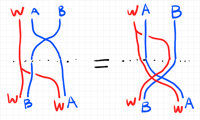
“見た目”からはいかにも成立しそうですが、示すには \sigma, \Delta, \alpha の性質を使います。

結果的に、 L_W は反ラックス対称モノイド関手になることが分かります。

準マルコフ関手としての掛け算関手

反ラックス・モノイド関手に仕立てた掛け算関手 L_W = (L_W, \delta, \varepsilon) が対称とも強調して反ラックス対称モノイド関手となることが分かりました。さらには、準マルコフ構造である対角射(の族)と廃棄射(の族)とも協調して、{反ラックス}?準マルコフ関手となることを見ましょう。({☓☓☓}? という書き方は☓☓☓部分は省略可能だということ。)

{反ラックス}?準マルコフ関手の条件は、「準マルコフ圏からなる2-圏」で述べました。再掲しておくと:


\forall A\in |\cat{C}|.\\
\quad F(\Delta_A);\delta_{A, A} = \delta_{F(A)}\;:\; F(A) \to F(A)\times F(A)\\
\:\\
\forall A\in |\cat{C}|.\\
\quad F(!_A);\varepsilon = \, !_{F(A)}\;:\; F(A) \to \I

 F = L_W の場合ならば:


\forall A\in |\cat{C}|.\\
\quad (\id_W\otimes\Delta_A);\delta_{A, A} = \delta_{W\otimes A}\;:\; W\otimes A \to (W\otimes A)\times (W\otimes A)\\
\:\\
 \forall A\in |\cat{C}|.\\
\quad (\id_W\otimes !_A);\varepsilon = \, !_{W\otimes A}\;:\; W\otimes A \to \I

これらも、モノイド圏の性質、\Delta, ! の性質(つまり、準マルコフ圏の性質)から示せます。

掛け算関手のさらなる性質

掛け算関手 L_W = (L_W, \delta, \varepsilon) は準マルコフ圏の2-圏 {\bf QMarkovCat}^\mathrm{oplax} の1-射であることが分かりました。さらに、2-圏 {\bf QMarkovCat}^\mathrm{oplax} の2-射 \boldsymbol{\delta}:L_W \Rightarrow L_W * L_W, \boldsymbol{\varepsilon} : L_W \Rightarrow \mathrm{Id}_{\cat{C}} で適切なものが見つかれば、この2-圏内の余モナドを構成できます。

モナドがあれば、余クライスリ圏が作れます。対象 W\in |\cat{C}| ごとに余クライスリ圏があるなら、全体としてインデックス付き圏が作れる可能性もあります。インデックス付き圏があるなら、ファイバー付き圏が作れます。

単に対象を掛け算するだけの操作が、けっこう複雑な構造物の事例となっているわけです。余モナド/余クライスリ圏/インデックス付き圏/ファイバー付き圏などの話はまたいずれ。

*1:圏の準マルコフ構造とは、各対象に余可換余モノイド構造が装備〈supply〉されていることです。